3 Microsoft Excel tips you can't live without

Microsoft Excel is the greatest "what-if" tool ever invented, and most people who use Excel are self-taught. As such, they learn things only when they need to perform a certain task or function.

Over the years, I have accumulated LOTS of Excel tips and tricks ^[1], and I teach the best ones in my Excel courses. Listed below are some of the tips I teach that people rave about over and over again. To work along with the tips below, click on this link to automatically download the Excel file ^[2], then click on the Home tab in the Office Ribbon.

If you use Excel or any Windows® program, you are probably already familiar with the Format Painter icon. It's the little icon that looks like a paint brush and is located in the Clipboard group of the Home tab on the Office Ribbon.

Most people already know how to use Format Painter. You use it to copy or "paint" the format of one cell or range of cells onto another. To illustrate, go to the NetIncome tab of the ExcelTipsWorkbook and work the following steps.

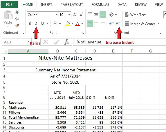
Click on Cell A19. This is the "source" cell.
Click on the Italics icon, then click on the Increase Indent icon . This makes the text in Cell A19 italics and indents it from the left.

Now let's suppose you want to apply this format to all the other cells in the worksheet that read "% of Revenue".

With your cursor still on Cell A19, click the Format Painter icon, then with your cursor click on Cell A21.

You see that Excel has copied the formatting of the source cell (A19) on to the destination cell (A21), but once you clicked on Cell A21, the formatting functionality went away. To retain the functionality, simply double-click on the Format Painter icon. Let's do it.

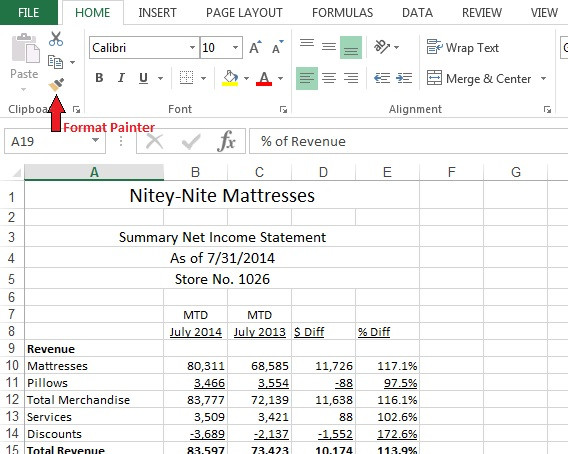
With your cursor on Cell A21, double-click the Format Painter icon, then click on Cells A23, A27, and all of the other cells in the spreadsheet that read "% of Revenue." Note: To see the actual numbers you may have to widen the cells.

To turn off the formatting functionality, click the Format Painter icon again or click the Escape key on your keyboard. Pretty cool, huh?

The Data Fill button is located on the bottom right corner of the cell or range of cells that you cursor is on. Among other things, it allows you to copy a formula without having to use the Copy and Paste icons in the Office Ribbon. In this next exercise, you will create a simple formula and copy it to the cells below it using Data Fill.

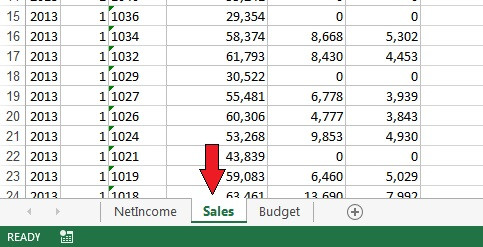
Click on the Sales tab of the ExcelTipsWorkbooks.xlsx file.
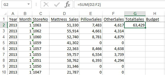
To sum the total sales by store and by month, type the following formula in Cell G2: =SUM(D2:F2)
Hold your cursor over the small black or green box at the lower right corner of cell G2. (Your cursor will turn to a + sign).

This activates the Data Fill functionality.

Click and drag the Data Fill box down to cell G6 and release.

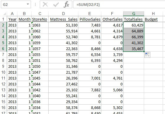
As you can see, dragging the Data Fill box copies cell G2 to the cells below it. But what if you have 650,000 rows of data to copy? It would take several minutes to click and drag that cell down to each of the cells below it. But it you double-click the Data Fill box, Excel will copy the formula down to the last cell in the list. Let's do it.

Click on Cell G6 and hold your cursor over the Data Fill box (your cursor turns to a + sign).
Double-click the Data Fill box.

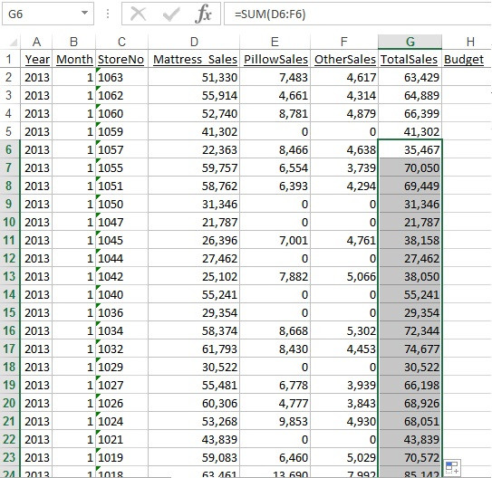
And presto! I've seen people spent countless time dragging the Data Fill button down when all they have to do is double-click it.

Many times, data is copied or linked from one database or spreadsheet to another, and the user has to work with whatever format in which it comes. In these situations, I encourage you to leave the data alone and write formulas to correct the data instead of correcting the physical data itself. If you write formulas around the data, it can change many times and the formulas will still work.

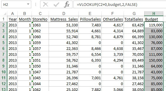
In the Sales tab, note that the values in the StoreNo field are formatted as text and not numbers. You can usually tell numbers are text when 1) the number is left-justified and/or 2) the numbers don't sum in a calculation. In this next exercise, you will look up the budget number for each store (contained in the Budget tab) and populate it on each row of the Sales tab.

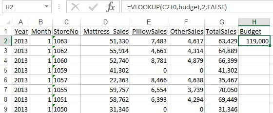
Click on Cell H2 of the Sales tab and write the following formula: =VLOOKUP(C2,budget,2,false)

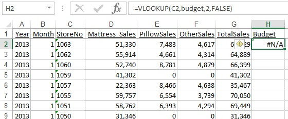
This formula looks up the budget for Store No. 1063 in the range called budget (this range is contained in the Budget tab). But you see that it returns a #N/A error. This is because the formula is looking Store No 1063 which is formatted as text, and comparing it to the first column of number in the budget range whose Store No. is formatted as a number.

In this situation, most people will either change all of the Store Nos. in the Sales tab to be a number, or change all of the Store Nos. in the Budget tab to be text. But the easiest way to make it work is to change the formula.

In the formula in cell H2, type "+0" immediately after the C2 reference (so the formula now reads =VLOOKUP(C2+0,budget,2,false).
Copy that formula down to all cells below it using the double-click Data Fill trick.